Download the UpLevered LBO Model (Excel)
Enter your email to unlock the template instantly.
Your LBO template is ready.
If the download doesn’t start, open the link in a new tab.
No spam. Unsubscribe anytime.
Let’s be real: learning how to build an LBO model isn’t just “nice to have” if you’re working in private equity, investment banking, or corporate finance— it’s absolutely essential. In middle market deals, which is where most buyouts actually take place, mastering leveraged buyout models can literally make or break your analysis. This comprehensive guide walks through the complete process, from initial assumptions to final returns calculations, with real-world examples and proven frameworks that PE firms actually use every day.
MM LBO models are a often a different beast entirely from mega-fund approaches. Deal sizes typically range from $25M to $500M in enterprise value, requiring way more hands-on modeling and serious attention to operational details. The stakes? Sky-high: a poorly constructed model can lead to covenant breaches, liquidity crunches, or worse—a complete loss of sponsor equity (and probably your job).
This guide provides a practitioner-focused approach to building robust LBO models. Whether you’re an investment banking analyst grinding through PE interview prep or a junior associate at a financial sponsor trying not to mess up your first model, this framework will seriously accelerate your modeling skills and deal execution confidence. For compensation benchmarking context, see Private Equity Salary 2026.
TL;DR — Building a Middle-Market LBO Model
Five steps, one template, done in under an hour:
- Entry Valuation — TEV from EBITDA × multiple, equity value via EV bridge
- Sources & Uses — match debt tranches + sponsor equity to purchase price + fees
- Debt Schedule — mandatory amort, cash sweep, revolver as plug
- Returns Analysis — exit equity → MOIC and IRR at base, upside, downside
- Sensitivity Tables — flex entry multiple, exit multiple, revenue growth, leverage
What ‘done’ looks like: Sources = Uses to the penny. Balance sheet balances every period. Cash flow bridge reconciles to debt paydown. IRR/MOIC move in the right direction when you stress assumptions.
Three common builds:
- Quick screen (30 min): simplified debt, no revolver, single exit case
- Full IC model (2–4 hrs): multiple tranches, cash sweep, management rollover, full sensitivity
- Lender case (1–2 hrs): downside-focused, covenant testing, recovery analysis
LBO Model Assumptions and Setup
Generally, position your key assumptions table at the model top for easy scenario testing.This single-source-of-truth approach allows rapid sensitivity analysis and prevents those dreaded #REF! from haunting your sheet.
Entry multiples: generally 6.0×–12.0× EBITDA, sector- and growth-dependent. Asset-light software can run high-single to low-teens (or use revenue multiples for earlier-stage profiles); industrials often sit mid- to high-single digits; services/healthcare land in between.
Deal size (EV): roughly ~$25M–$500M for typical MM examples (sweet spot for hands-on experience).
Revenue growth: model realistic 5%–15% ranges. Many MM companies grow organically ~3%–8%; bolt-ons add incremental growth. Anything >20% needs explicit justification and stress testing.
Leverage: total 4.0×–6.0× under post-’22 credit conditions; senior 3.0×–4.5×, with sub/mezz filling the gap. Present actual tranche pricing in the debt schedule.
Rates (illustrative): TLA ≈ SOFR+300–400 bps; TLB ≈ SOFR+450–550 bps; mezz ≈ 10%–12% all-in.
Exit multiple: start by matching entry and test ±1.0× to bracket valuation risk.
Hold period: 5–7 years (fund-cycle dependent). Taxes: 25%–30% blended, jurisdiction-dependent.
Equity Purchase Price = EV − Net Debt
Net Debt = Total Debt − Cash
For MM entry multiples smaller add-ons lean towards the lower end of the valuation range while recurring-revenue, larger companies being toward the higher end. It is also heavily dependant on sector and growth profile. Software companies usually command higher multiples (even can based on revenue / subscriber multiples), while traditional manufacturing can sit lower,as product lines can die and capex requirements are higher.
Revenue growth rates should reflect realistic projections of 5%-15% annually or lower, GDP-lever if conservative / looking at the out years. Aggressive assumptions above 20% require extraordinary justification and serious stress testing (because your MD will definitely grill you on it). Most MM companies grow organically at 3%-8%, with bolt-on acquisitions adding incremental growth.
Standard holding period assumptions span 5-7 years for PE funds, aligning with fund lifecycles and LP return expectations (because LPs get kinda angry when you hold too long). Tax rate assumptions should incorporate blended federal and state rates of 25%-30%, adjusting for geographic footprint and entity structure.
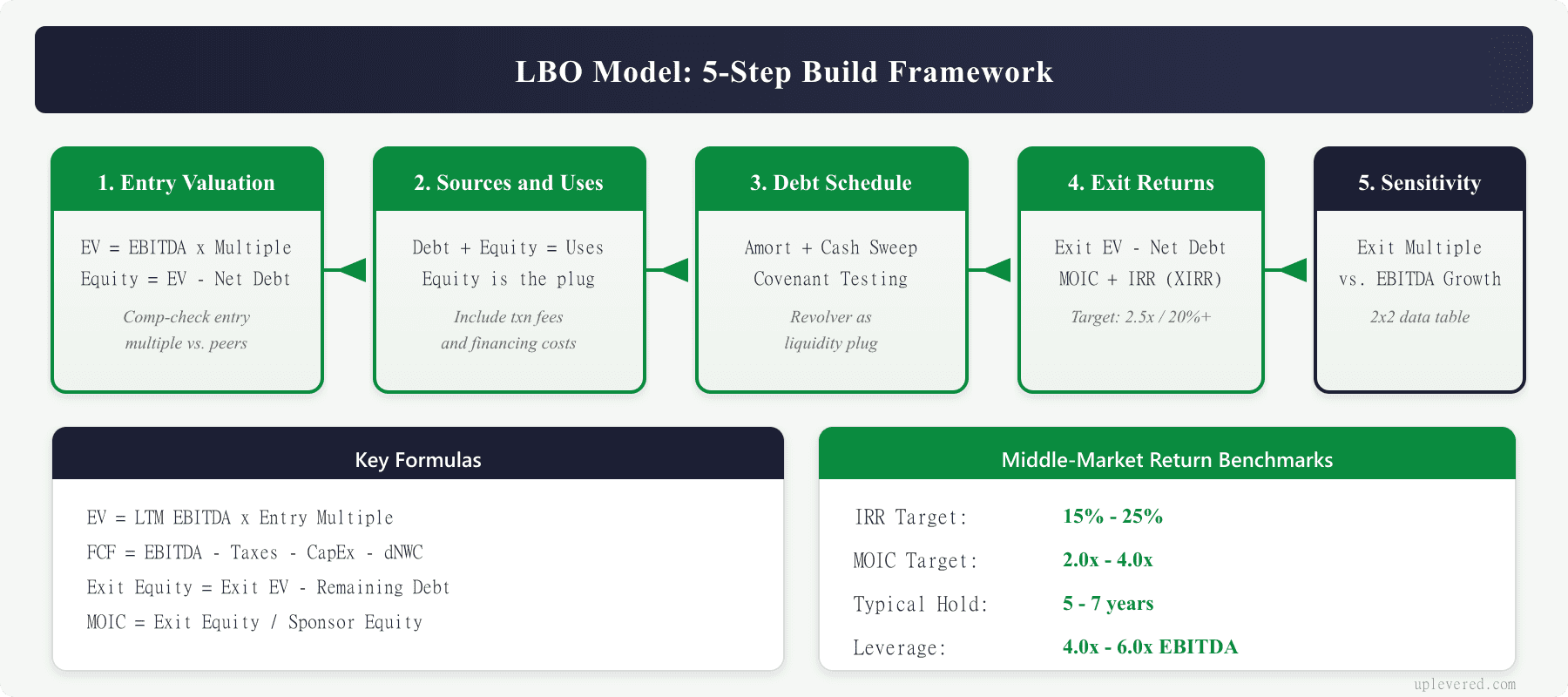
How to Build an LBO Model: 5-Step Framework
Master these five core steps for any MM LBO analysis. Each step builds upon previous calculations and assumptions, creating an integrated financial model that actually captures deal dynamics and return drivers.
Focus on keeping clean for the sake of your comrades. Broken Excel formulas / links absolutely destroy model integrity and create downstream errors that compound throughout the analysis. So Use consistent formatting and color coding throughout your model—blue for inputs, black for calculations, green for outputs.
Step 1: Calculate Entry Valuation
Enterprise Value equals LTM EBITDA multiplied by Entry Multiple assumption. This foundational calculation drives literally every subsequent analysis (so don’t screw it up).
Example calculation: $10M EBITDA × 10.0x = $100M Enterprise Value
Subtract existing debt and add cash balance to determine Equity Purchase Price. Most MM deals structure on a cash-free, debt-free basis with normalized working capital, simplifying the transaction.
“Growing revenue usually consumes cash; model ΔNWC explicitly or you’ll overstate FCF.”
Equity Purchase Price = Enterprise Value - Net Debt (Total Debt - Cash)
Cross-check valuation against precedent transactions and trading comparables. Entry multiple assumption significantly impacts returns—a 1.0x multiple difference can swing IRR by 400-600 basis points in typical MM structures.
Step 2: Create Sources and Uses Table
Uses side captures every single dollar required to close the transaction: purchase price plus transaction fees plus financing costs. Transaction fees typically range 2%-4% of deal value for MM transactions, including investment banking fees, legal fees, and due diligence costs (lawyers don’t work for free, unfortunately).
Sources side shows funding structure: senior debt plus subordinated debt plus sponsor equity. Target 40%-60% equity contribution for stable cash flow businesses. Higher leverage works for asset-heavy or recession-resistant sectors (but don’t get too aggressive or you’ll regret it later).
Sources = Uses
Senior Debt + Subordinated Debt + Sponsor Equity = Purchase Price + Fees + Financing Costs

Note: Modeled on a cash-free, debt-free basis with normalized NWC; equity is the plug so Sources = Uses.
Financing fees represent 2%-3% of total debt amount, covering original issue discount, legal fees, and arrangement fees. Sponsor equity becomes the plug to balance sources equals uses—this automatic calculation prevents manual errors; everyone loves a good plug.
EV = $100M; Net Debt = $10M  → Equity Purchase Price = $90M
Fees: Transaction $3M; Financing $1M
Uses = $90M + $3M + $1M = $94M
Sources: Senior $55M; Sub $15M; Sponsor Equity = $24M (plug)
Check: $55 + $15 + $24 = $94M ✓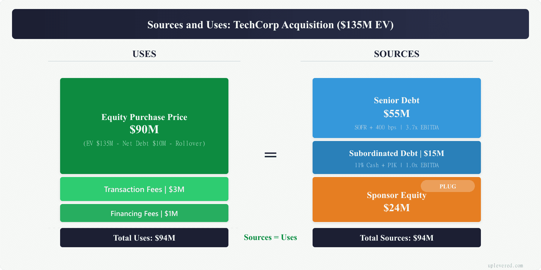
Step 3: Build Financial Projections and Debt Schedule
Forecast income statement for 5-7 year holding period, starting with revenue projections and flowing through to net income. Calculate free cash flow using the standard formula:
Free Cash Flow = EBITDA - Cash Taxes - CapEx - Change in Net Working CapitalNote there is way more nuance to Free cash flow (FCF) then this, but shown for the sake of simplicity
📊 2026 Middle-Market Debt Terms
Current market clearing rates for $50M-$500M EV deals in 2026. Ranges are illustrative; confirm current market terms for your deal.
| Tranche | Pricing (Spread) | Max Leverage | Amortization |
|---|---|---|---|
| Senior / TLA | SOFR + 350-450 bps | 2.5x – 3.5x | 5.0% – 7.5% |
| Unitranche | SOFR + 550-650 bps | 4.0x – 5.5x | 1.0% |
| Mezzanine | 11% – 13% (Cash+PIK) | Turns of < 1.0x | Bullet |
Cash sweep provisions require 50%-75% of excess cash flow to debt paydown after meeting minimum liquidity requirements. Include covenant testing for Total Leverage and Interest Coverage ratios—most MM deals include step-downs over time.
Step 4: Model Exit Scenarios and Returns
Exit Enterprise Value equals Exit Year EBITDA multiplied by Exit Multiple assumption. Conservative modeling assumes exit multiples match entry multiples, with upside cases testing 1.0x-2.0x multiple expansion scenarios (but don’t count on multiple expansion to save a bad deal).
Exit Equity Value = Exit Enterprise Value - Remaining Debt BalanceCalculate IRR using Excel’s XIRR function with proper dates for cash flows. Avoid using Excel’s IRR function—it assumes annual cash flows and produces totally inaccurate results for stub / different period ending dates.
MOIC (Multiple of Invested Capital) equals Exit Proceeds divided by Initial Equity Investment. Target returns for MM deals: 15%-25% IRR, 2.0x-4.0x MOIC range over 5-year holding periods (anything less and you need to put your ops team to work).
Step 5: Conduct Sensitivity Analysis
Test key variables systematically: entry multiple, exit multiple, EBITDA growth, and leverage assumptions. Create data tables showing IRR across different scenarios using Excel’s Data Table functionality (and yes, you need to know how to do this).
Get Deal Flow Bullet — free, every Friday.
One email a week — real deal frameworks and technical breakdowns from a middle-market practitioner. No fluff.
Include base case (most likely), upside case (+20% EBITDA performance), and downside case (-20% EBITDA performance) projections. Stress test debt capacity and covenant compliance under adverse scenarios—MM companies face way higher volatility than large-cap peers, as they have less resources to weather the same storms.
Most sensitive variables typically rank: (1) Exit multiple, (2) EBITDA growth rate, (3) Entry multiple, (4) Leverage level. Focus sensitivity analysis on the first two drivers for maximum impact (because that’s where the real value creation happens).
Paper LBO 10-Minute Method
📝 The 60-Second Paper LBO
Memorize this logic for interviews. Do not use a calculator.
*Tip: If you pay down half the debt over 5 years, your MOIC automatically jumps ~0.5x. Mentioning this proves you understand cash flow.
Quick mental math approach for initial deal screening enables rapid evaluation without full model builds. Investment banking analysts and PE professionals use this technique during live deal discussions and interview situations (and it’s absolutely crucial for interviews).
Step 1: Calculate purchase price using EBITDA × entry multiple assumption
Step 2: Estimate debt capacity at 4x-6x EBITDA for conservative screening
Step 3: Determine equity requirement as purchase price minus debt capacity
Step 4: Project exit value using future EBITDA × exit multiple
Step 5: Calculate returns as exit proceeds ÷ equity investment
Example: $10M EBITDA company at 10x entry multiple requires $100M purchase price. Assuming 6x debt capacity provides $60M financing, leaving $40M equity requirement. Target 3x MOIC requires $120M exit proceeds minimum (basic math, but surprisingly effective).
Required Exit Enterprise Value = (Target MOIC × Equity Investment) + Projected Debt Balance
$120M = (3.0x × $40M) + $60M
This method provides directional guidance within 10-15% of detailed model results, sufficient for initial screening and interview scenarios (and way better than fumbling around with a calculator).

⚠️ Common Modeling Traps (Reality Checks)
Avoid these specific errors that destroy model integrity. For a deeper breakdown, see LBO modeling traps.
-
🛑 Circular References
Circular references between cash balance and interest calculations absolutely destroy inexperienced modelers (and honestly, will make you question your life choices at 2 AM). Look, just solve this by separating beginning-of-period cash from end-of-period calculations, or use Excel’s iterative calculation feature with extreme caution (though let’s be real, just avoid circularity altogether because nobody has time for that nightmare).
-
🛑 Financing Fee Amortization
Forgetting to include financing fee amortization in your debt schedule? Yeah, that’s gonna understate your true interest expense big time. Most financing fees amortize over 5-7 year terms, creating this non-cash expense that absolutely impacts covenant calculations (and trust me, your MD will definitely notice if you miss this – and they won’t be sending you a friendly Slack message about it).
-
🛑 Wrong Debt Pricing
Using wrong interest rates for different debt tranches literally destroys accuracy faster than you can say “refinancing.” Senior debt, subordinated debt, and mezzanine debt carry totally different pricing based on risk profile and security position. Revolver pricing differs from term loan pricing (this isn’t some optional knowledge you can Google later – this is the fundamentals, people).
-
🛑 Cash Sweeps & Amortization
Neglecting cash sweep mechanics and mandatory amortization? That’s how you end up with overly optimistic leverage profiles that make your model look like fantasy football projections. Most MM credit agreements require aggressive debt paydown when performance exceeds thresholds (because lenders aren’t idiots, despite what your VP might mumble during all-hands meetings).
-
🛑 Aggressive Growth Assumptions
Overly aggressive revenue growth assumptions above 20% annually basically require you to channel your inner Steve Jobs with extraordinary justification. Conservative modeling protects against covenant breaches and liquidity shortfalls during market downturns (and trust me, downturns always happen – usually right when you’re finally feeling confident about your model).
-
🛑 Working Capital Drag
Ignoring working capital impacts on free cash flow? That’s how you create dangerous cash flow timing mismatches that’ll haunt your dreams. Growing companies typically consume cash through receivables and inventory build (basic working capital dynamics that somehow everyone forgets, even though it’s literally Finance 101).
-
🛑 Transaction & Integration Costs
Missing transaction costs and integration expenses straight-up understates your required capital needs. Budget 1%-3% of purchase price for systems integration, management changes, and operational improvements (because integration definitely isn’t free, and those consultants aren’t working for exposure).
-
🛑 Covenant Stress Testing
Failing to stress test covenant requirements under adverse scenarios? That’s how you set yourself up for seriously unpleasant surprises that make Sunday Scaries look like a vacation. Model covenant compliance using 15%-25% EBITDA decline scenarios (because bad things absolutely happen to good companies, and Murphy’s Law is basically a fundamental principle of finance).
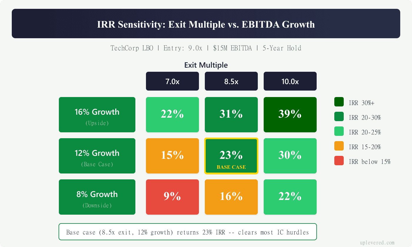
Middle Market LBO Example: TechCorp Acquisition
Target: Software company with $15M LTM EBITDA, 85% recurring revenue, 25% EBITDA margins, serving mid-market customers across North America (classic SaaS play).
Entry multiple: 9.0x EBITDA = $135M Enterprise Value, reflecting software premium but MM discount versus venture-backed peers (because you’re not buying the next Salesforce here).
Debt structure: $75M Term Loan at SOFR+500 bps (5.0x EBITDA), $25M revolver for working capital flexibility. Total leverage of 6.7x EBITDA pushes covenant boundaries but reflects strong cash conversion (aggressive but not totally crazy).
Sponsor equity: $35M (26% of purchase price), providing adequate downside protection while maximizing leverage benefits (the sweet spot for returns).
Revenue growth: 12% annually through organic expansion and bolt-on acquisitions, with EBITDA margin improvement to 28% via operational efficiencies (realistic but requires execution).
Exit assumptions: Year 5 with $25M projected EBITDA, 8.5x exit multiple reflecting normalized market conditions (conservative exit multiple assumption).
Exit Enterprise Value = $25M × 8.5x = $212.5M
Less: Remaining Debt Balance = ($45M)
Exit Equity Proceeds = $167.5M
Returns: 2.8x MOIC, 23% IRR over 5-year hold period, exceeding MM return thresholds and justifying aggressive leverage structure (solid returns that would make LPs happy).
Sensitivity Analysis: 2×2 Matrix
Create matrix showing IRR sensitivity to key variables for comprehensive scenario analysis. X-axis represents Exit Multiple range (7.0x – 10.0x), Y-axis shows EBITDA Growth Rate (8% – 16%) (because these are the variables that actually matter).
EBITDA Growth / Exit Multiple | 7.0x | 8.5x | 10.0x |
|---|---|---|---|
16% | 22% | 31% | 39% |
12% | 15% | 23% | 30% |
8% | 9% | 16% | 22% |
Base case intersection: 9.0x exit multiple, 12% growth = 23% IRR meets target return thresholds (right where you want to be).
Downside scenario: 7.0x exit multiple, 8% growth = 9% IRR approaches return floor, requiring operational improvements or extended hold period (not great, but not catastrophic).
Upside scenario: 10.0x exit multiple, 16% growth = 39% IRR generates exceptional returns, justifying aggressive entry valuation (home run territory).
Use conditional formatting to highlight target return thresholds—green for IRR >20%, yellow for 15%-20%, red for <15%. This visual approach seriously accelerates investment committee discussions (and makes your presentation look professional).
How-To: LBO Model Best Practices
Use consistent cell formatting and color coding system throughout your model. Blue cells indicate inputs requiring assumptions, black cells show calculations and formulas, green cells highlight key outputs and returns (stick to this system religiously).
Build assumption-driven model with input cells clearly marked and grouped logically. Single assumption table at model top enables rapid scenario testing without hunting through multiple tabs (your future self will thank you).
Include error checks and data validation throughout model structure. Use Excel’s ISERROR function to catch circular references and #DIV/0! errors before they propagate (because #REF! errors make you look amateur).
Create executive summary dashboard on first tab showing key metrics: entry multiple, leverage ratios, projected returns, and covenant compliance. Busy partners and investment committees appreciate summary-first presentation (because nobody has time to dig through your 47-tab model).
Document all key formulas and calculation methodologies using Excel comments. Future users (including yourself in six months) will absolutely appreciate clear explanations of complex calculations.
Test your model with extreme scenarios to check for errors and logical inconsistencies. Input 50% revenue decline or 15x entry multiple to identify weak formulas or circular references (stress testing reveals everything).
Save multiple versions during build process with clear naming conventions. Model corruption during complex builds creates totally unnecessary rework and deadline pressure (learned this the hard way).
Include internal links to navigate between model sections efficiently. Hyperlink buttons improve user experience and professional presentation quality (small details matter).
Common LBO Model Traps
| Trap | What Goes Wrong | How to Catch It | Fix |
|---|---|---|---|
| Exit multiple baked into entry | You assume the same or higher exit multiple as entry, inflating returns | Compare entry and exit multiples — if exit ≥ entry with no thesis, it’s a red flag | Default exit = entry multiple. Justify any expansion with operational improvement or re-rating catalyst. |
| Sources ≠ Uses | Transaction doesn’t balance — usually a missed fee, rounding error, or double-counted rollover | Check S&U totals. They must match to the penny. | Build a S&U check cell that shows the difference. Flag if ≠ 0. |
| Working capital ignored | Model assumes zero ΔNWC, overstating FCF and debt paydown | Check if NWC changes flow through cash flow statement | Add ΔNWC line in operating cash flow. Link to balance sheet NWC items. |
| Circular reference panic | Revolver/cash sweep creates circular logic, model breaks or iterates forever | Enable iterative calculation in Excel (File → Options → Formulas → Enable iterative calculation) | Use a circular breaker switch. Or model revolver as beginning-of-period balance. |
| Over-leveraging the cap structure | Total debt/EBITDA exceeds realistic levels for MM deals, lender wouldn’t fund it | Check total leverage ratio against market benchmarks (4–6× for MM) | Size debt to realistic coverage ratios: ≤6× total leverage, ≥1.5× FCCR for MM deals. |
LBO Model Audit Checklist
Before submitting any LBO model — to your MD, your interviewer, or your IC memo — run through this list:
Sources & Uses
- Total sources = total uses (to the penny)
- All fees included (financing fees, advisory fees, transaction expenses)
- Management rollover flows through both sides
- Minimum cash included in uses if applicable
Balance Sheet
- BS balances every period (total assets = total liabilities + equity)
- Goodwill = purchase price – net tangible assets (simplified) or from PPA
- Deferred financing fees amortize over debt life
- NWC ties to revenue/COGS assumptions
Cash Flow
- Cash flow bridge: EBITDA → less taxes → less capex → less ΔNWC → less interest → FCF
- FCF drives mandatory debt paydown, then sweep, then revolver repayment
- Cash balance never goes negative (revolver draws if needed)
Debt Schedule
- Mandatory amortization matches term sheet (e.g., 1% p.a. for Term Loan B)
- Cash sweep applies to correct tranches in correct priority
- Revolver balance never exceeds facility size
- Interest rates match assumptions (fixed vs floating + spread)
Returns
- Exit equity = exit TEV – net debt at exit
- MOIC = exit equity ÷ sponsor equity invested
- IRR calculation uses correct timing (entry at t=0, exit at t=n)
- Returns move in expected direction when stressing assumptions
Sensitivity
- Entry multiple, exit multiple, revenue growth, and leverage each have sensitivity tables
- No circular errors or #REF values in any scenario
- Downside case still services debt (DSCR > 1.0×)
Frequently Asked Questions
Most sponsors underwrite to ~15–20% net IRR as a floor, with mid-20s%+ considered strong. Thresholds vary by vintage, risk profile, leverage, and hold length. Sub-15% can clear for lower-risk profiles or strategic angles, but it’s uncommon for traditional buyouts.
Typical post-’22 structures land at ~4.0×–6.0× total debt / EBITDA, with senior 3.0×–4.5× and sub/mezz filling the gap. Sector, cash-flow stability, asset base, and lender appetite drive the exact mix.
Default to cash-pay for healthy credits. Use PIK only in special situations (e.g., stressed credits, heavy reinvestment, junior capital). PIK increases debt balances, can pressure covenants, and complicates documentation—model it explicitly per tranche.
Use quarterly projections or a 13-week cash-flow for WC-intensive or seasonal businesses. Translate AR/Inv/AP days into dollar balances, and model the revolver/ABL dynamically with a facility cap and borrowing base where relevant.
Start with entry multiple, then test ±1.0× to bracket valuation risk. Tie expansion/compression to specific factors (mix shift, growth durability, margin/quality improvements, public comp cycles). Avoid assuming expansion without a value-creation thesis.
Model each tranche: base rate + spread, amortization, mandatory vs. optional prepayments, cash-sweep % after a minimum liquidity buffer, and covenant tests (leverage, interest coverage). Calculate interest on BoP or average balances to avoid circularity.
Reflect a real amend-and-extend path: amendment fees, margin step-ups, tighter baskets, potential PIK toggles on junior paper, equity cure, cost-out plan, and (often) a longer hold. Make each change explicit so returns reconcile.
Only if they’re central to the thesis. If included, model timing (close date), purchase price allocation, integration costs, incremental ΔNWC, and synergy timing (revenue/cost). Otherwise, keep the base case organic and show bolt-ons as upside.
Related Technical Guides
- Enterprise Value vs. Equity Value — The EV bridge that feeds your entry valuation
- Net Operating Working Capital (NOWC) — Why ΔNWC matters more than most analysts think
- Distribution LBO Case Study — Apply what you’ve learned: a full $150M MM deal walkthrough
- 5 Common LBO Modeling Traps — The errors that silently destroy your returns math
- Middle-Market Definition — Deal sizes, buyer types, and why MM operates differently
- Private Equity Value Creation Levers — Revenue growth, margin expansion, and deleveraging quantified
Update Log
- March 2026 — Added TL;DR, model traps table, 20-item audit checklist, cross-links, update log
- February 2026 — Fixed MOIC calculation, updated meta description, standardized formatting
- January 2026 — Updated assumptions and benchmarks to 2026 market conditions
- September 2025 — Original publication
Stay sharp. Subscribe to Deal Flow Bullet.
Weekly PE frameworks, deal analysis, and career intel for middle-market practitioners. Free, every Friday.
Last updated: February 2026