Distribution businesses live and die by working capital. In this case study and Excel walkthrough, we tackle a $150 million distributor LBO to see what makes these deals unique. We’ll walk through the downloadable hands-on model to show how improving day-to-day operations, like vendor rebates and route density, drive returns. Download the Excel model now to follow along.

Private Equity Case Study (MM): $150M Distribution LBO — Step-by-Step + Model

Learn to crack a private equity case study for a distribution LBO—fast. Inside: a minute-by-minute approach, an ABL / borrowing base primer, a clean paper LBO grid, and a value-creation bridge. Links to Value-Creation Levers, Interview Strategy, and our Resume guide are included.
No email required — full model download below.

Download the Distribution Mini-LBO (Excel) — Free

Why distribution LBOs are different

Distribution is a working-capital sport. Cash gets tied up in AR and inventory while suppliers still want to be paid. The cash conversion cycle (CCC) = AR days + Inventory days − AP days; small day-shifts unlock (or consume) real dollars and move the revolver in/out. Everything below is geared to make that dynamic obvious in your model.

Rebates (make P&L ≠ cash obvious)

What they are: Vendor volume discounts that reduce COGS on the P&L now but pay in cash later. The gap sits in rebates receivable (generally excluded from ABL collateral). EBITDA is not cash flow, so—don’t count on rebates to service debt until they hit cash.

Model it like this (simple and explicit):

• P&L: show COGS (gross) and less: rebates (separate line → transparent GM%).
• Balance sheet: add Rebates Receivable (grows when you accrue, shrinks when paid).
• Cash flow: make sure Δ Rebates Receivable flows inside ΔNWC.
• Borrowing base: exclude rebates receivable from eligible AR.

Quick mental math: Every $1.0M of rebate accrual lifts EBITDA now but $0 cash until it pays.

Why this matters: EBITDA can run ahead of cash in rebate-heavy periods; lenders exclude rebate receivables from ABL, so they won’t fund debt service until paid.
Model checkpoint: You should see a Rebates Receivable line, ΔNWC capturing its change, and BB that doesn’t count it; recheck FCCR when rebates receivable climbs.

Asset-Based Lending (ABL) & availability (define the constraint)

What it is: A revolver secured by working capital.

Borrowing Base (BB): 0.85 × eligible AR + 0.50 × eligible Inventory → Availability = MIN(BB, Facility Cap).

Borrowing Base (BB): 0.85 × eligible AR + 0.50 × eligible Inventory → Availability = MIN(BB, Facility Cap)

Unused availability: Availability − Revolver EOP.

The trap: Sales/AR surge → BB up, but you draw more to fund it; unused availability can shrink. The facility cap can bind before BB does.

Model moves:

• Build a BB block with advance rates and cap.
• Compute Unused Availability; traffic-light troughs (e.g., < ~$3mm = red).
• Interest on average revolver; revolver = cash plug to min cash.

Tiny example: AR + $5.0M → BB + $4.25M (85%). If you need the cash, you’ll draw $4.25M and unused availability likely falls.

Why this matters: In distributors, availability (not theoretical BB) is often the binding liquidity constraint.
Model checkpoint: Show BB, Cap, Availability, Unused Availability, and Peak Revolver; flag cap-bound periods (BB > Cap) and low headroom.

Working-capital intensity (AR / Inventory / AP) (give a cheat sheet)

Cash-Conversion-Cycle (CCC) basics: CCC = DSO + DIO − DPO. Shorter = better. Growth without turn improvements consumes cash and forces revolver draws.

Per $100M cheat sheet (order of magnitude):

• AR ±5 days ≈ ±$1.37M cash (5/365 × $100M sales).
• Inventory ±10 days ≈ ±$2.05M cash if COGS ≈ $75M (25% GM).
• AP ±5 days ≈ ±$1.03M cash (5/365 × $75M).

Model moves:

• Drive AR/Inv/AP $ from DSO/DIO/DPO each year.
• Flow ΔNWC to cash; link AR/Inv to BB; AP reduces cash need.
• Add a before/after mini-table (e.g., 45/45/20 → 40/35/25).

Why this matters: Tiny day shifts move millions of dollars; without better turns or longer payables, growth eats cash.
Model checkpoint: Run a mini-sensitivity (±5d DSO, ±10d DIO, ±5d DPO), watch ΔNWC, revolver plug, FCCR, and Unused Availability react.

Route density & delivery optimization (convert ops into EBITDA)

What it is: More drops per route + tighter territories lower delivery cost (fuel, drivers, wear). It’s a low-capex lever.

How to model (honest version):

• Phase SG&A % reduction (e.g., +30–50 bps EBITDA margin over 12–24 months).
• Include small enablement spend in opex/capex (routing software, dispatch rules).
• Savings flow EBITDA → FCF → lower revolver / higher FCCR.

Tiny example: On $200M sales, 30 bps SG&A save = $0.6M EBITDA; in a 10% cash interest world, that’s meaningful covenant headroom.

Why this matters: Routing tweaks create repeatable EBITDA, improving debt service without big capex.
Model checkpoint: Confirm savings aren’t double-counted; ensure they hit EBITDA and then reduce revolver / lift FCCR over time.

Inventory optimization & product mix/scale (cash + margin)

Two buckets, two effects:

1. Turns (cash today):
   • DIO ↓ 10 days can free $2–3M per $100M sales (assume ~25% GM).
   • Model: lower Inventory days → ΔNWC inflow; note BB may shrink but liquidity improves (less borrowing).
2. Mix & scale (margin every day):
   • Private label / price discipline / scale rebates can add +50–150 bps GM.
   • Model: gradual GM% lift and rebate % step-up; rebates still lag in cash (receivable grows first).

Guardrails: Don’t over-tighten—stockouts can hit revenue and raise DSO (disputes, short ships).

Why this matters: Turns give cash today; mix/scale add margin daily—together they drive faster deleveraging.
Model checkpoint: When DIO falls, check Inventory $↓, BB↓, Unused Availability↑; model GM% and rebate % ramps with a rebates receivable lag in ΔNWC.

Base Case Frame (the Deal in Numbers)

Let’s set up the base case. Industrial Inc. is a regional industrial distributor with $25 million in LTM EBITDA being acquired for 6.0× EV/EBITDA, or $150 million enterprise value. We’ll finance it with a combination of equity and debt, including an asset-based revolver to fund working capital. Key deal parameters:

Deal Frame:

Metric	Year 0 (2025)	Year 5 (2030)
EBITDA	$25M	~$38M
EV / EBITDA	6.0×	6.0×
Enterprise Value	$150M	~$230M
Net Debt	$75M	~($20M)
Sponsor Equity	($80M)	$245M

Other Considerations:

• Transaction Fees: 3% of purchase enterprise value
• Debt Structure:
  • $75 million senior term loan (@9% interest); optional prepayments with excess cash
  • $5 million ABL revolver draw (@6% interest)
    • $30 million revolver limit, tied to borrowing base (85% of AR + 50% of Inventory); $5MM drawn as close
• Tax Rate: 25% (for cash tax calculations)
• Capex: ~2–3% of sales (maintenance capex to keep operations running)
• Working Capital Assumptions: AR Days 40 (improve to 35 by exit); Inventory Days 45 (improve to 40); AP Days 20 (stretch to 25). These improvements are phased in over the hold period.
• Rebate Policy: Vendor rebates net against COGS in EBITDA, but cash receipt lags (rebates create a receivable that collects with delay).

This base case assumes no immediate multiple arbitrage – entry and exit multiples are both ~6.0×. A strong ops team at your firm is proficient at value creation, which will drive returns from EBITDA growth and debt paydown (operations and working capital wins). Now, onto the fun part – building the model to see how it plays out.

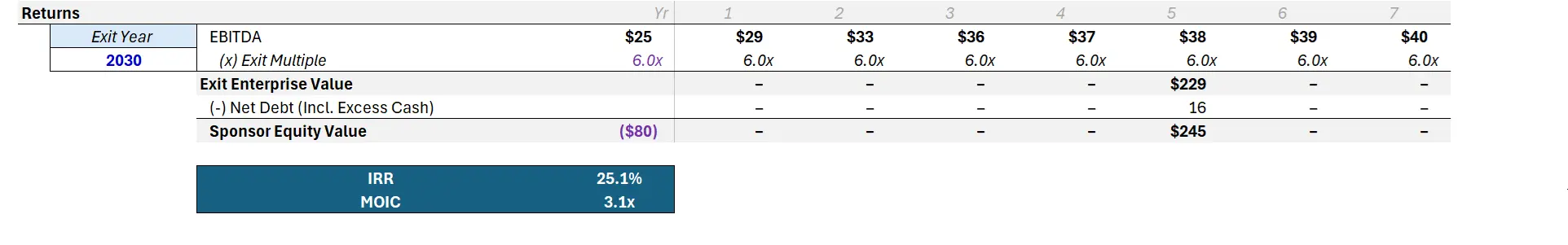
Overview of base case returns:

Metric	Year 5 (2030)	Industry Average Targets
Internal Rate of Return (IRR)	25.1%	25.0%
Multiple of Invested Capital (MOIC)	3.1×	3.0×

Excel Walkthrough— Build the Model

In this section, we’ll build a simplified LBO model step-by-step, focusing on the mechanics unique to a distributor. You can follow along in the provided Excel, which has an “Assumptions & Questions” tab and a “Mini_LBO” tab where the model lives. We’ll highlight key formulas and logic as we go. Buckle up – you’ve got about an hour to complete this template, and by the end you’ll deeply understand the moving pieces of a $150M distribution LBO.

Sources & Uses

We start with the Sources & Uses table – the transaction’s funding roadmap. This lays out where the money comes from (sources) and how it’s spent (uses) to close the deal.

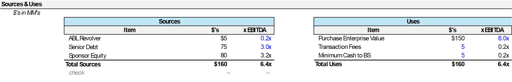
Notice the term loan and revolver 3.2× EBITDA = sponsor equity of 3.2× – a moderate leverage deal. .

Uses (total = $160M, 6.4× EBITDA):

• Purchase Enterprise Value: $150M (6.0× on $25M EBITDA)
• Transaction Fees: $5M (legal, banking, diligence). Note fees and min cash are equity-funded
• Minimum Cash to Balance Sheet: $5M (Day-1 operating cushion)

Sources (total = $160M, 6.4× EBITDA):

• Sponsor Equity: $80M (3.2×) — funds the $5M fees and part of purchase price
• Senior Debt (Term Loan @ ~9%): $75M (3.0×)
• ABL Revolver Draw (@ ~5–6%): $5M (0.2×) — plugs to minimum cash

At-a-glance leverage at close (x EBITDA):

• Gross debt: 3.2× (3.0× term + 0.2× ABL)
• Equity: 3.2×
• Total sources/uses: 6.4×

Why this matters: This layout makes three things explicit: (1) fees are equity-funded, (2) the revolver is a small plug to meet min cash, and (3) you’re underwriting moderate leverage (3.2×) with plenty of ABL headroom for working-capital swings.

Model checkpoint:

• Sources = Uses tie to $160M.
• xEBITDA column totals 6.4× on both sides.
• Fees shown in Uses and covered by equity (not by ABL).
• Opening balances after close: Cash ≈ $5M, Term Loan $75M, Revolver $5M, Equity $80M → Net debt ≈ $75M (3.0×).

One check: after funding, the company’s opening balance sheet will have ~$5 M cash (minimum), $75 M term debt, $5 M revolver debt drawn, and $80 M equity. Net debt is $75 M ($80 M less $5 M cash). This will be close to matching the $150 M EV, but note there is usually a slight difference because fees/min cash distort a bit.

---

Borrowing Base & Availability (ABL)

The borrowing base (BB) caps how much we can draw on the ABL based on working-capital collateral. It’s collateral math first, then a facility cap.

Eligibility & formulas

• BB = 85% × eligible AR + 50% × eligible Inventory
  (explicitly exclude rebates receivable and any ineligibles/reserves)
• Availability = MIN(BB, Facility Cap)
• Unused Availability = Availability − EoP Revolver

Your model (what it shows)

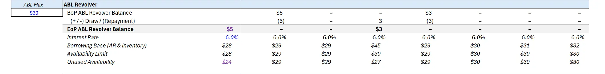
• Facility cap: $30mm
• Close (2025A): BB ≈ $28mm → Availability ≈ $28mm; EoP ABL = $5mm → Unused ≈ $23–24mm
• AR +30d shock (2028P): AR balance jumps; BB ≈ low-to-mid $30s but the cap binds, so Availability ≈ $29–30mm; EoP ABL ≈ $3mm → Unused ≈ $27mm
• Post-shock: BB normalizes (~$29–32mm) and availability remains under the $30mm cap

Why it matters

• In a collections shock, collateral (BB) can rise, but availability is still capped—so the headroom you can actually use is what matters.
• In your base build, unused availability stays ample (>~$25mm), even when the cap binds. If revolver usage rises faster than collateral, unused can tighten even as BB climbs.

Model checkpoints

• Rebates receivable: shown on the BS, excluded from BB, and ΔRebates flows through ΔNWC.
• Debt schedule shows BB, Availability (cap-limited), Unused, and EoP ABL (e.g., close: ~$28 / ~$28 / ~$24 / $5; shock: ~$35 / ~$29–30 / ~$27 / $3).
• Revolver is the cash plug; optional term prepay occurs only when ABL = 0 and cash > min.

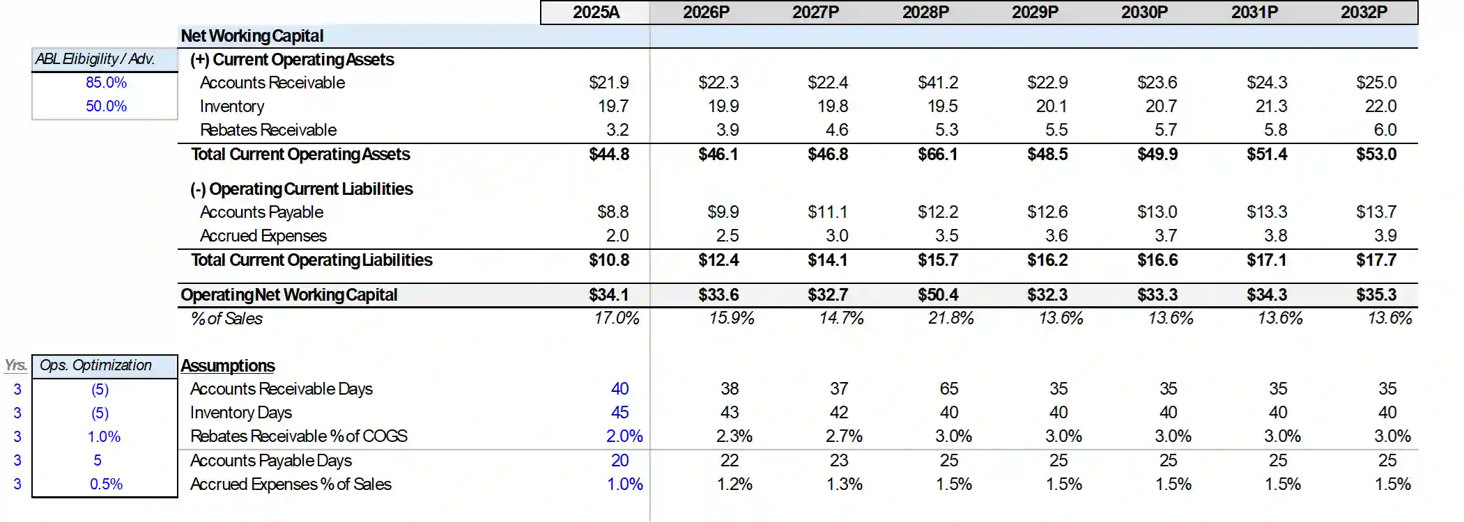
Working Capital Days Schedule

This section converts day counts → dollar balances and then computes ΔNWC → cash.

Formulas (annual):
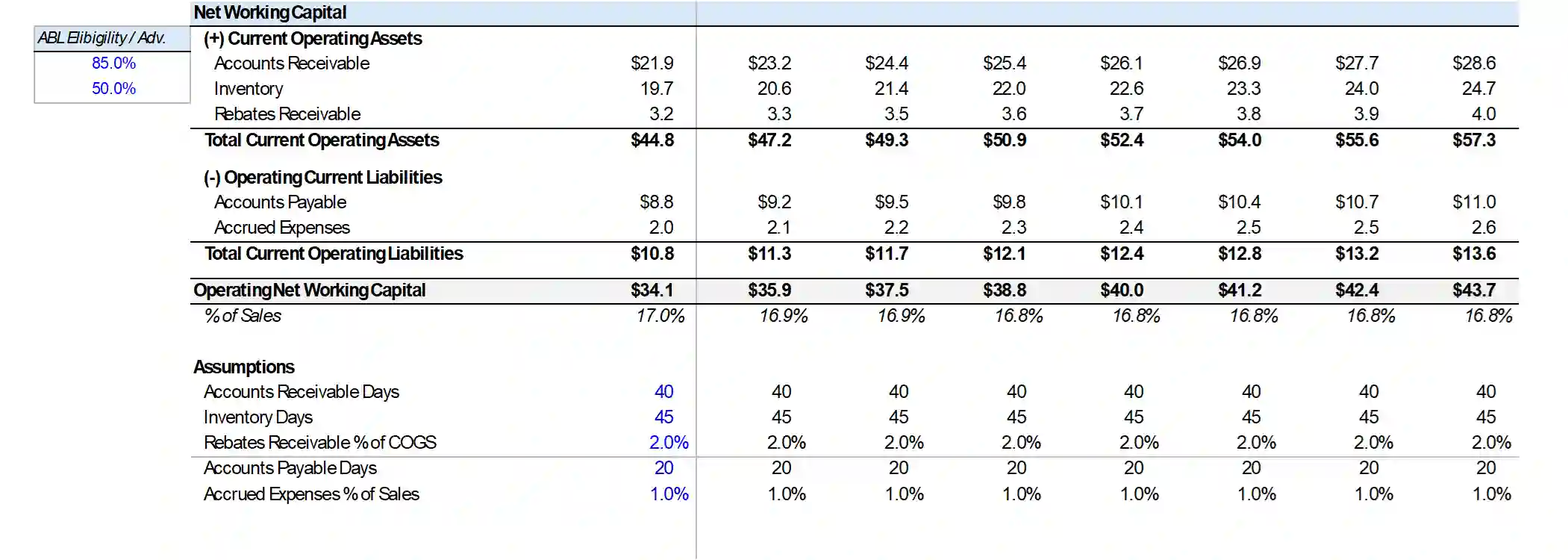
AR = Revenue × DSO/365 | Inventory = COGS × DIO/365 | AP = COGS × DPO/365
Operating NWC = AR + Inventory + Rebates Receivable − AP − Accrued Exp.
ΔNWC = NWCₜ − NWCₜ₋₁ (cash use if positive, source if negative)

Pre-improvement snapshot (2025A)

• Days: AR 40d, Inventory 45d, AP 20d
• Rebates receivable: 2.0% of COGS (on BS, excluded from ABL, cash lags P&L)

Target glide path (post-improvement)

• AR steps down to 35d by 2029+
• Inventory tightens to 40d and holds
• AP stretches to 25d and holds
• Rebates receivable ramps to 3.0% of COGS by 2028 and holds (still excluded from ABL)

One-year shock (2028P)

• Collections slow: AR jumps to 65d for one year, then normalizes

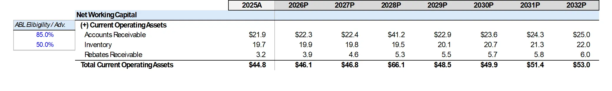
What your model shows (balances, $mm)

• AR: 21.9 → 22.3 → 22.4 → 41.2 (shock) → 22.9 → 23.6 → 24.3 → 25.0
• Inventory: 19.7 → 19.9 → 19.8 → 19.5 → 20.1 → 20.7 → 21.3 → 22.0
• AP: 8.8 → 9.9 → 11.1 → 12.2 → 12.6 → 13.0 → 13.3 → 13.7
• Rebates receivable: 3.2 → 3.9 → 4.6 → 5.3 → 5.5 → 5.7 → 5.8 → 6.0
• Operating NWC: 34.1 → 33.6 → 32.7 → 50.4 → 32.3 → 33.3 → 34.3 → 35.3
  (% of sales on sheet: 17.0% → 15.9% → 14.7% → 21.8% → 13.6% …)

Cash implications (ΔNWC → cash):

• 2028 shock: NWC +~$18mm (32.7 → 50.4) = ~$18mm cash outflow, drives a revolver draw
• 2029 normalization: NWC −~$18mm (50.4 → 32.3) = ~$18mm cash inflow, repays revolver and enables optional term prepay
• Across the hold, the glide 40/45/20 → 35/40/25 steadily releases cash vs. a no-improvement case

Why this matters: In distribution, tiny day shifts move millions. The one-year AR spike shows how quickly liquidity can tighten even when the underlying business is fine.

Model checkpoints (tie-outs)

• Days drive dollars: AR/Inv/AP balances come only from DSO/DIO/DPO.
• ΔNWC feeds FCF directly (cash use if positive).
• Rebates receivable sits on BS, excluded from ABL; Δ rebates is included in ΔNWC.
• Revolver = cash plug: draws in 2028, repays in 2029 (min cash maintained).
• Keep a mini before/after banner visible: 2025A → 2029+: AR 40→35 | Inv 45→40 | AP 20→25.

Change in NWC — one-paragraph explainer

Each year, ΔAR + ΔInventory − ΔAP flows into the cash bridge as ΔNWC. Improving AR days or Inventory days creates inflows (balances shrink relative to sales). Extending AP days is also an inflow (you’re borrowing from suppliers). Conversely, growth that builds AR/inventory is a cash outflow. That’s why the model subtracts ΔNWC in FCF: if working capital increases, it consumes cash; if it falls, it releases cash—critical in Year 1 post-close and in the 2028 shock → 2029 normalization sequence.

---

Free Cash Flow Calculation (how to read this block)

This block converts the P&L into cash and then shows how cash moves through the debt stack. We start at EBITDA, subtract cash taxes, cash interest, capex, and the change in operating NWC (AR, inventory, AP, and rebates receivable), to get FCF before debt service. Then we take mandatory amortization, let the revolver act as the cash plug, and use any residual to make optional prepayments on the term loan (subject to cash minimums and no revolver balance).

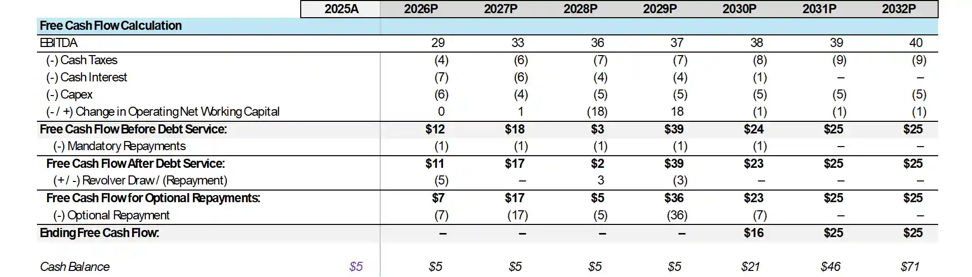
Note the 2028P AR shock (ΔNWC outflow) triggers a revolver draw; the 2029P normalization reverses it and accelerates optional term prepay.

Key mechanics

• Rebates reduce COGS (so margin improves) but cash is delayed — the increase in rebates receivable is included in ΔNWC (use of cash).
• Interest is calculated on average balances; it steps down as debt is repaid.
• Capex is maintenance-like (low for distributors; your model rounds it to ~$4–$6MM/yr).

What your model shows (numbers line up with your table)

• EBITDA grows from $29MM → $40MM from year 1 to year 5.
• Cash taxes run about 25% of EBIT (rising with profits).
• Capex stays steady at ~$4–$6MM per year.
• ΔNWC drives the story:
  • 2028P shock: AR days jump for one year → ΔNWC = (18) (i.e., $18MM outflow), so FCF before debt service dips to $3MM and the revolver draws $3MM to fund the gap.
  • 2029P normalization: AR days snap back → ΔNWC = +18 (inflow), FCF before debt service rebounds to $39MM and the revolver repays (3).
  • Outside the shock year, ΔNWC is modest (~$1MM outflow each year) as AR/Inv tighten and AP stretches (your glide path 40/45/20 ➜ 35/40/25).
• After amortization, you generate $11–$25MM of FCF after debt service.
• Optional prepay sweeps excess cash to the term loan whenever (i) the revolver is $0 and (ii) cash > minimum. That’s why you see (7), (17), (5), (36) in the prepay row — the 2029P surge is the ΔNWC reversal being swept to debt.
• Ending cash builds once debt is largely down: ~$5MM flat early, then $21MM / $46MM / $71MM as optional prepay winds down.

Plain-English takeaway: in a distributor, small changes in days swing ΔNWC by eight figures, which flips revolver usage and optional paydowns year-to-year even when EBITDA is steady. Your one-year AR spike makes that visible without breaking the model.

Model guardrails (built-in)

• Revolver is the plug. It draws to cover cash shortfalls and repays on excess cash, but never exceeds availability or goes below $0; minimum cash is respected.
• Optional prepay logic. Only fires when EoP ABL = 0 and cash > min. Prepay is capped at (BOP term + current mandatory) so you can’t over-repay.
• ΔNWC includes rebates. Rebates receivable are excluded from the ABL BB but included in ΔNWC, so a rebate ramp is a cash use even as EBITDA rises.

If something looks off:
• Unused availability < 0? Your draw is being capped by the facility—check the BB and cap.
• Term prepay happening while ABL > 0? Sweep condition is misapplied—ensure prepay is gated by EoP ABL = 0.
• Cash building while ABL > 0? You’re likely hitting min cash or availability; confirm the revolver repay logic.

---

Debt Paydown

Objective: See how cash flows through the revolver (ABL) and term loan, and confirm the sweep only pre-pays term when the revolver is at $0 and cash > min.

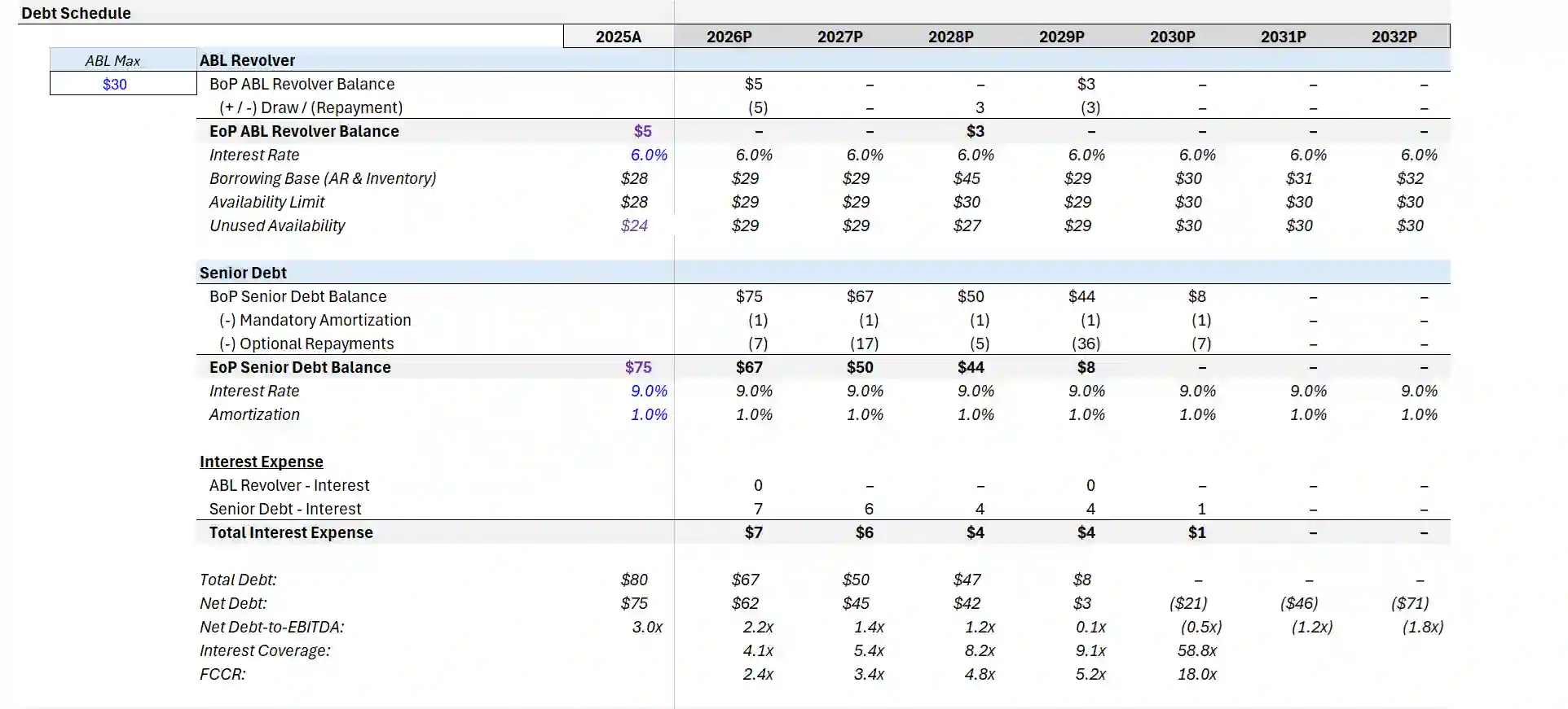
Pay attention to whether and when the revolver fully pays off and if any term prepayment happens (it should only prepay when revolver = $0 and excess cash beyond $5M exists – as we set in our logic).

How the model works

• Revolver is the plug. Draws to keep min cash in shock years; repays first when there’s excess cash. Never exceeds availability (MIN[BB, facility cap]) and never drops below $0.
• Mandatory amortization: 1%/yr on the term loan (typical).
• Optional sweep: After revolver = $0 and cash > $5mm, excess goes to term prepay (capped at remaining principal so you can’t over-repay).
• Interest on average debt: Term @ 9%, ABL @ 6%, both on average balances for the year.

What your model shows (year-by-year highlights)

• 2025A: ABL starts $5mm and repays to $0; term goes $75 → $67mm (-$1mm mandatory, -$7mm optional).
  Interest ≈ $7mm; Net Debt/EBITDA ~ 3.0x; FCCR 2.4x; Unused availability ~$24mm.
• 2026P: Strong FCF; term $67 → $50mm (-$1mm mandatory, -$17mm optional).
  Interest ≈ $6mm; leverage 2.2x; FCCR 3.4x.
• 2027P: Term $50 → $44mm (-$1mm mandatory, -$5mm optional).
  Interest ≈ $4mm; leverage 1.4x; unused availability ~$29mm.
• 2028P (AR +30d shock): Working-capital outflow forces EoP ABL ≈ $3mm; sweep pauses.
  Availability limit binds at $30mm; unused availability still ~$27mm; interest stable.
• 2029P (normalization): Revolver repays (3) to $0; big ΔNWC inflow drives term prepay (-$36mm) → term $44 → $8mm.
  Interest ≈ $4mm; Net Debt/EBITDA ~0.1x; FCCR 5.2x.
• 2030P–2032P: Term is cleared ($8 → $0), cash builds ($21 / $46 / $71mm), Net Debt turns negative (net cash).
  Interest drops to ≈ $1mm then ~0; coverage ratios become very high.

Do this (reader tasks)

• Confirm sweep logic: no term prepay in 2028P while EoP ABL > 0; big prepay occurs in 2029P once ABL hits $0 and cash > min.
• Check interest math: Total interest ≈ 9% × avg Term + 6% × avg ABL (your totals fall $7 → $1mm as debt declines).
• Validate headroom: Unused availability never negative; EoP ABL ≤ Availability each year.
• Watch covenants: FCCR stays above ~1.1× (your path: 2.4× → 5.2× → 18.0×); Net Debt/EBITDA trends down to <1.0× and then net cash.

Why it matters

Distributors live and die by working-capital swings. The schedule shows the classic ABL pattern: the revolver zigzags with AR/Inventory timing, while the sweep retires term debt aggressively once liquidity normalizes—driving most of the multiple-safe return via deleveraging rather than heroic growth.

---

Stress Test — AR +30 days for one year

Objective: Show how a one-year collections slip ripples through ΔNWC, revolver usage, and availability (cap binding).

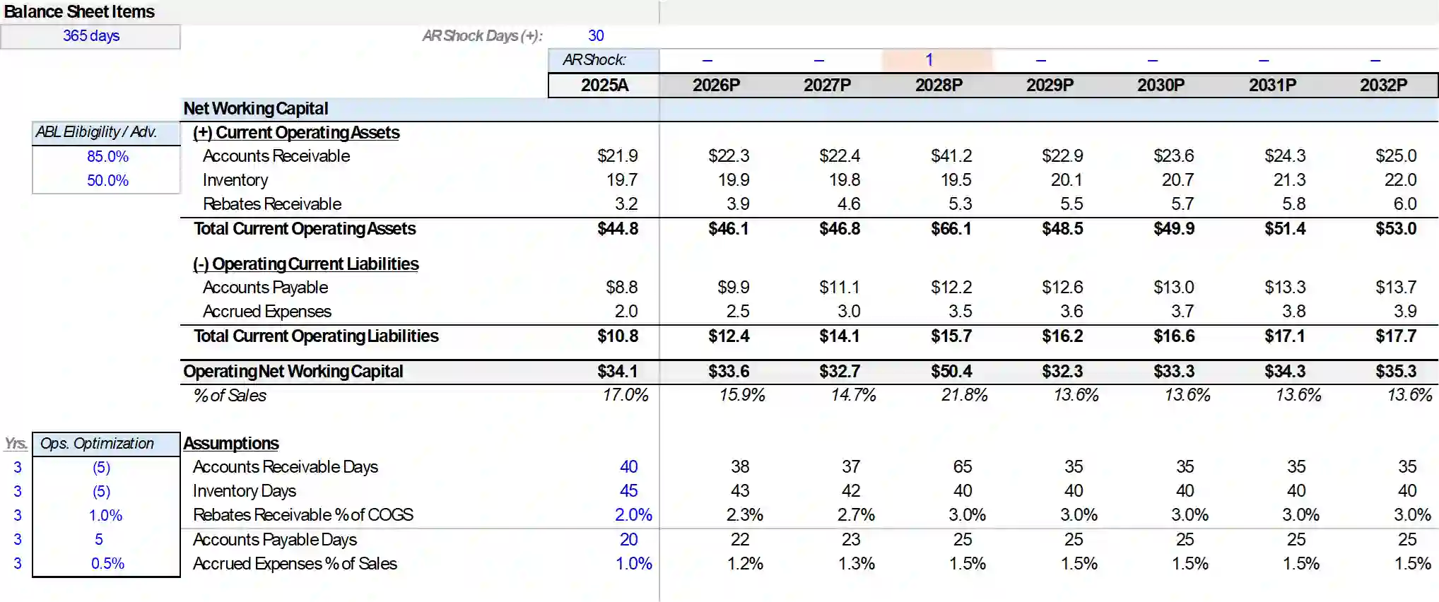
Notice that although our borrowing base went up with AR, the constraint was actually the availability limit and the business’s own need for cash – a stark reminder that base ≠ cash in hand.

Do this

• Set ARShock = 30 (applies to 2028P only).
• Recalculate; keep all other assumptions the same.
• Note ΔNWC, FCF before/after debt, EoP ABL, Unused availability, and IRR/MOIC.

What happens in your model

• AR days jump 40 → 65 in 2028P; AR balance spikes to ~$41mm (from ~22mm).
• ΔNWC ≈ +$18mm (use of cash) → FCF before debt dips to ~$3mm.
• The revolver draws ~+$3mm (cash plug) to keep min cash.
• Borrowing base rises to ~$45mm, but the facility cap ($30mm) binds:
  • Availability limit ≈ $30mm
  • EoP ABL ≈ $3mm
  • Unused availability ≈ $27mm (ample headroom)
• 2029P normalization: AR days revert; ΔNWC ≈ −$18mm (inflow) → revolver repays (3) to $0, and a large term prepay (−$36mm) fires.
• Returns take a modest hit (timing only): you should see a small IRR dip with MOIC unchanged at exit.

Checkpoints (tie-outs)

• ΔNWC row: ~+18 in 2028P, −18 in 2029P.
• Debt schedule: BB ~45 / Availability 30 / Unused ~27 / EoP ABL ~3 in the shock year.
• Covenants: FCCR remains comfortably > 1.2× throughout (your path sits multiple turns above).
• No over-advance: EoP ABL ≤ Availability; Unused never negative.

Why it matters

In ABLs, collateral can rise while usable headroom is capped—what matters is unused availability and the revolver’s ability to bridge timing shocks without tripping covenants. The next year’s normalization often over-delivers cash, accelerating term paydown and restoring trajectory.

What happens when AR days spike? First, AR balance balloons because customers are slower to pay – cash gets sucked out of the business to fund this receivable growth. Our borrowing base will increase (more AR means more collateral), but that’s not exactly good news – it just means the bank will lend us more because we need it. In Year 3 of our model, AR days go from ~35 to 65 for the shock. The borrowing base formula yields a much higher number (say it jumps from ~$30M to ~$45M). However, remember the facility cap is $30M, so any base beyond $30M doesn’t help – we’re still limited to $30M of total revolver borrowing.

The company will draw heavily on the revolver to cover payables and expenses during this cash crunch. In our model, we see the revolver peak usage in Year 3. Unused availability tightens: even though the base was theoretically $45M, the cap means max $30M credit; if we end up borrowing, say, $25M, then only $5M is left undrawn. The liquidity headroom shrinks, which is dangerous – one more hit and you’re at the ceiling.

This AR shock also dents IRR. Why? Because the extra borrowing incurs more interest and the principal won’t get fully repaid until the customer pays up in Year 4. That means higher debt at exit or less cash to pay down term debt. In our scenario, the equity IRR might drop a few percentage points versus the base case due to this one-year shock. It’s a classic distribution risk: growth or an external shock can force borrowing and delay deleveraging, harming returns.

When things normalize in Year 4, AR days go back down, releasing cash (as customers catch up payments). The revolver then gets paid back down quickly with that inflow. However, some damage is done in terms of interest cost and lost time.

---

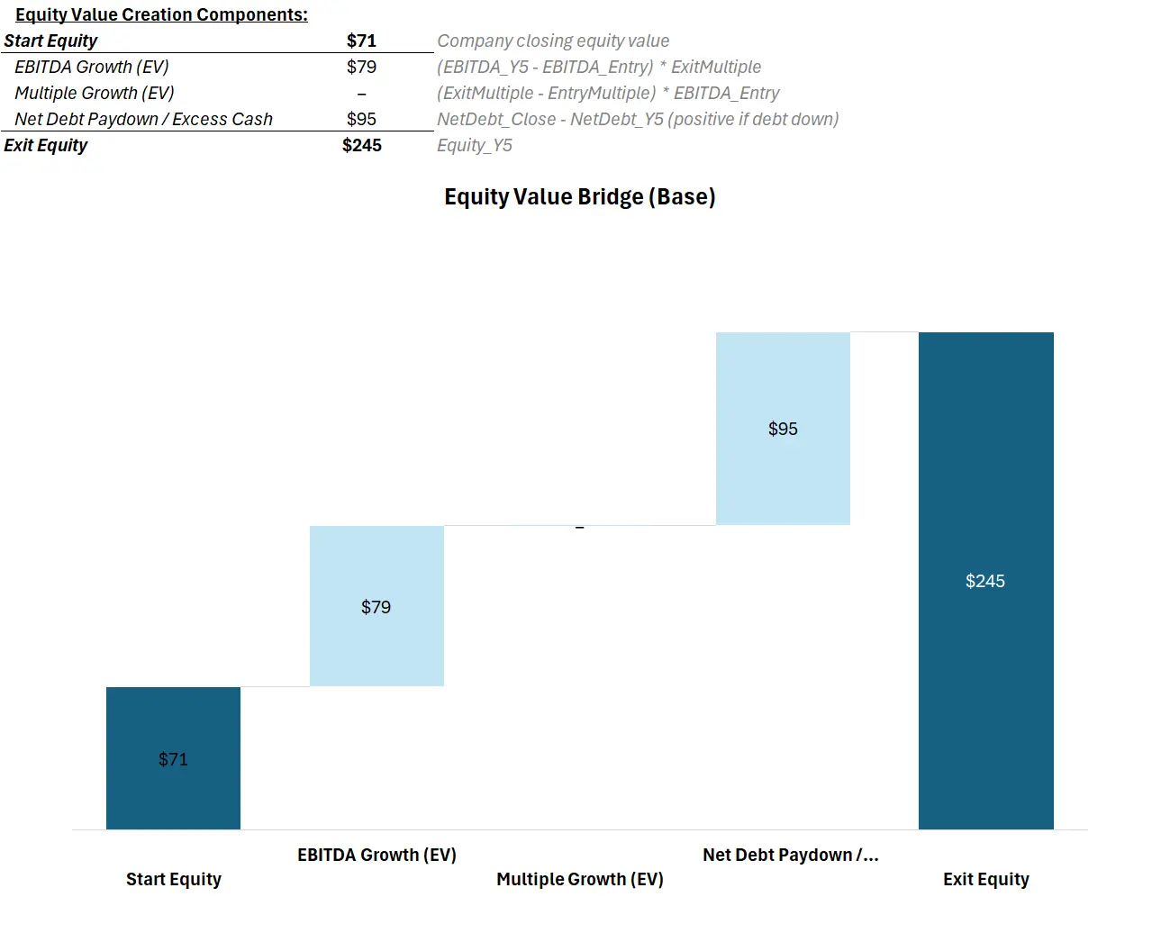
Equity Value Bridge

Let’s step back and see how the value is created in this deal. The Equity Value Bridge breaks down the sources of equity gain from entry to exit: how much came from EBITDA growth, how much from multiple change, and how much from debt paydown.

Essentially shows: how equity grows from close → exit via three levers:

1. EBITDA growth (EV)
2. Multiple change (EV)
3. Net debt paydown / excess cash

Formulas (no cell refs):

• Start Equity = equity value at close (TEV − net debt at close)
  Note: because fees/min cash are equity-funded, Start Equity can be < sponsor equity check. That’s why your bridge starts at ~$71mm even though total equity raised at close was higher.
• EBITDA Growth (EV) = (Exit EBITDA − Entry EBITDA) × Exit multiple
• Multiple Δ (EV) = (Exit multiple − Entry multiple) × Entry EBITDA
• Net Debt Paydown / Excess Cash = NetDebt_Close − NetDebt_Exit
• Exit Equity (check) = sum of the above (should tie to model’s exit equity)

Your base case (matches the chart):

• Start Equity: $71mm
• EBITDA Growth (EV): $79mm
• Multiple Δ (EV): $0mm (you keep the same multiple at entry and exit)
• Net Debt Paydown / Excess Cash: $95mm
• Exit Equity (tie): $245mm

The bridge adds cleanly: 71 + 79 + 95 = 245 (no plug), confirming the math.

Why these bars move (distribution context):

• EBITDA growth comes from pricing/rebate capture (rebates net against COGS), gross-margin lift, and route/Inventory Optimize efficiencies (lower SG&A and DIO).
• Deleveraging is powered by steady FCF and working-capital release (AR/Inv down, AP up) after the one-year AR shock normalizes.
• Multiple is held flat—typical for steady distributors—so returns are earned operationally.

Do this (reader task):

• Confirm Exit Equity on the bridge equals the equity value in your Year-5 outputs.
• Flip the exit multiple scenario (±1.0×) and watch only the Multiple Δ bar move.
• Toggle the AR shock off and note how the Net Debt Paydown bar grows (more cash swept to term).

Why it matters:

This bridge mirrors the classic LBO value levers: EBITDA growth, multiple arbitrage, and debt paydown. It forces you to quantify what drove the equity return. In distribution deals, you’ll typically see a hefty portion from EBITDA growth (via margin expansion and maybe some tuck-in acquisitions) and good chunk from debt paydown (if operations throw off cash). Multiple expansion is often not a given in a steady industry like this, so you have to earn your return operationally.

Paper LBO — sanity check (does the full build make sense?)

Before declaring victory, we ensure our detailed model makes sense with a back-of-envelope “paper LBO” and key credit metrics. This is a sanity check section.

Quick math (back-of-envelope):

• Equity in: ~$80 sponsor check (fees/min cash funded with equity).
• Equity out: $245mm (Year-5, 6.0× exit on ~$38mm EBITDA minus ~$16mm net debt).
• MOIC: $245 / $80 ≈ 3.1× (matches model).
• IRR: ~25% over 5 years (your returns block shows 25.1%).

Liquidity & covenants:

• Peak revolver draw: $5mm at close; $3mm in the AR-shock year; otherwise $0.
• Min unused availability: ~$24mm (close), ~$27mm during the shock—headroom never negative even when the cap binds.
• FCCR (min): ~2.4× (well > typical 1.1× threshold).
• Binding constraint: neither covenant nor availability actually trips; availability comes closest in the shock year, so that’s the watch item.

What moves the return:

• Deleveraging and EBITDA growth are the big bars in the bridge; multiple is flat.
• The one-year AR spike pulls IRR down a touch (timing), but normalization the next year over-delivers cash and accelerates the sweep—MOIC is basically unchanged.

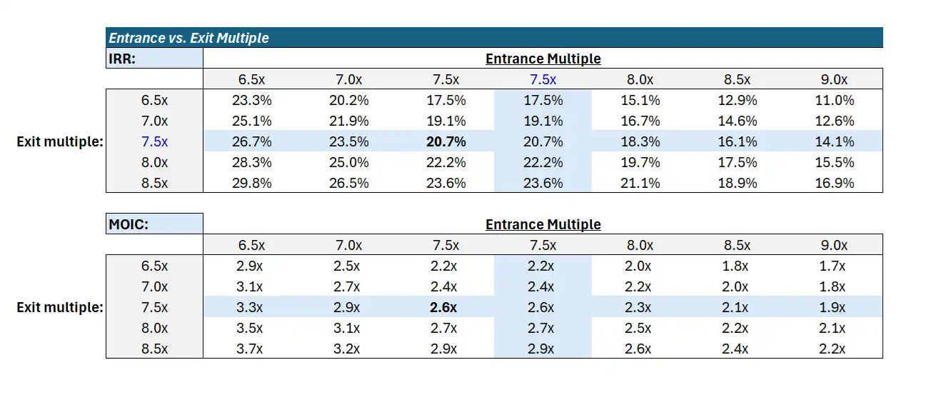
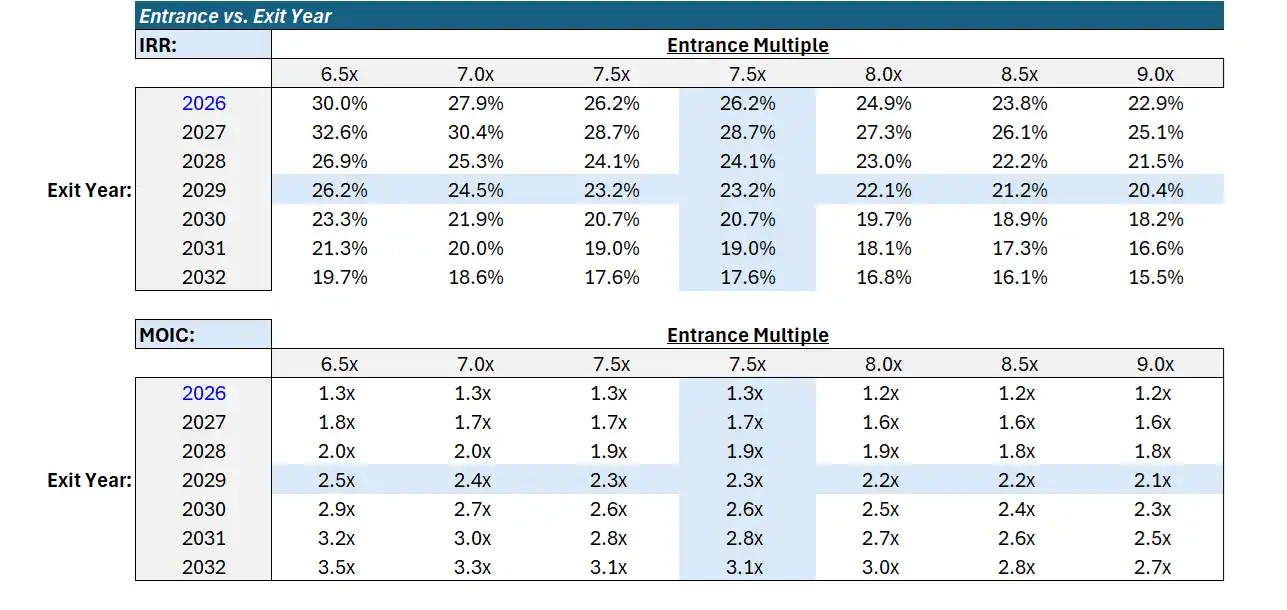
Sensitivities (how to read your grids):

• In the multiple grid, moving ±1.0× on exit typically shifts IRR by ~3–5 pts and MOIC by ~0.2–0.4×.
• In the exit year grid, slipping exit by a year trims IRR (same MOIC over longer time); pulling exit forward boosts IRR.
• Highlight the cell corresponding to your base case so readers can orient quickly.

Screenshot cues:

• Place the Returns strip (MOIC/IRR table) first, then the two sensitivity heatmaps. Caption:
  “Back-of-envelope matches the build: ~3.1× / ~25% at 6.0× exit. Headroom stays positive even in the AR shock; FCCR never breaches.”

One-liner conclusion:
The detailed model passes the paper-LBO sniff test: 3.1× MOIC / 25% IRR with ample ABL cushion and healthy FCCR—returns are earned via operations and deleveraging, not multiple expansion.

If the paper LBO math doesn’t roughly match the model’s outputs (for MOIC/IRR), something’s off. But assuming it’s in line, we’ve validated the model.

Finally, consider the exit: at 6.0× exit on the higher EBITDA, the buyer’s getting a company with better working capital metrics and lower debt. Would you pay more than 6× for that improvement? Possibly – and that could be upside if we assumed any multiple expansion. But as disciplined underwriters, we don’t bank on it; it’s gravy if it happens.

---

Hands-On Tasks

Download the model and work through these mini-exercises. Take a screenshot of each result (top of the relevant block) and jot 1–2 lines of explanation.

1) Borrowing base at close

Do: Using the AR & inventory balances at close, compute the ABL borrowing base and availability.
Formula: BB = 85% × AR + 50% × Inventory; Availability = MIN(BB, $30mm cap); Unused = Availability − EoP ABL.
Expect: BB ≈ $28–29mm; Availability ≈ $28–29mm; EoP ABL = $5mm; Unused ≈ $24mm.
Screenshot: Borrowing-base table (AR/Inv, advance %, cap, unused).

2) Extra inventory tightening (liquidity impact)

Do: Improve inventory days by 10 (e.g., Year 1 to 35d, gliding to ~25d by Year 5).
Explain: You should see a one-time ΔNWC inflow, lower ABL BB, less revolver usage, and earlier term prepay. Liquidity improves even though the BB shrinks.
Screenshot: Working-capital days (before/after) and FCF block showing ΔNWC change.

3) Collections shock: AR +30 days for one year

Do: Set ARShock = +30 for the designated shock year.
Report: ΔNWC (use), peak EoP ABL (~$3mm), and minimum unused availability (~$27mm). Note that the $30mm cap binds, but headroom stays positive.
Screenshot: WC table (with 65d AR) and debt lines for Availability / Unused / EoP ABL.

4) Sweep logic check (prepay only when ABL = 0)

Do: Verify there’s no term prepay in the shock year (ABL > 0), and a large prepay when AR normalizes (ABL = 0 and cash > min).
Expect: Prepay pauses in the shock year; resumes next year with a big sweep.
Screenshot: Debt schedule (EoP ABL, optional prepay row).

5) Build the equity value bridge by hand

Do: Using model outputs, compute:

• Start Equity (equity value at close)
• EBITDA Growth (EV) = (Exit EBITDA − Entry EBITDA) × Exit multiple
• Multiple Δ (EV) = (Exit − Entry multiple) × Entry EBITDA
• Net Debt Paydown / Excess Cash = NetDebt_Close − NetDebt_Exit
  Tie-out: Sum to the model’s Exit Equity (≈ $245mm in base). Your bars should be ~$71 / $79 / $0 / $95 → $245.*
  Screenshot: The bridge chart/table.

6) Paper-LBO sanity

Do: With just entry/exit numbers, compute MOIC and IRR, and pull: min FCCR, min unused availability, peak revolver.
Expect (base): ~3.1× MOIC, ~25% IRR; FCCR ≥ ~2.4×; unused availability stays positive even in the shock year; peak ABL ≈ $3–5mm.
Decide: Which was the binding constraint at the trough—availability or FCCR? (In this case, availability came closer to binding.)

What to turn in (1 page)

• 6 small screenshots (one per task)
• A bullet under each with the number(s) you observed and your one-sentence explanation

Tip: If something doesn’t reconcile, check the guardrails: revolver as the plug, prepay only when ABL = 0 and cash > min, rebates receivable excluded from BB but included in ΔNWC.

---

Recommendation — invest or pass?

So, do we invest in Industrial Inc. at 6.0x, or pass? Our recommendation: a cautious invest. The base case delivers a solid ~3.1× MOIC / ~25+% IRR over five years, driven by achievable operational tweaks (better pricing, working capital cleanup) rather than heroic assumptions. The company’s cash generation is strong enough to deleverage steadily – fixed charge cover stays above 2.0× and ABL availability never fully maxes out in our projections.

Key risks revolve around liquidity and execution: a single large customer stretching payments could strain the revolver, and margin improvement requires discipline in pricing and routing.

We propose two mitigants: (1) Lock in pricing durability via multi-year contracts or surcharges so that gross margin gains (like that 300 bps from rebate and pricing initiatives) stick. (2) Maintain ABL headroom by aggressively managing receivables – maybe offer early-pay discounts to customers or use credit insurance for big accounts. And (3) invest in route optimization tech to cement those cost savings in deliveries (higher route density translates to permanent margin lift). With these in place, the downside (liquidity crunch or margin squeeze) is manageable, and the upside – a well-oiled distributor that could even sell for a premium – is attractive.

In summary, this distribution LBO isn’t a get-rich-quick story; it’s a steady operational play. But by turning operational dials, we create a path to a respectable return. For hands-on investors who know how to squeeze cash from the balance sheet, Industrial Inc. is a buy.

Further Reading

• LBO Modeling Traps: 5 That Can Kill Your IRR – UpLevered (2025) – Highlights common pitfalls like underestimating working capital needs (e.g., high-growth “cash traps” in distributors) and how to avoid them.
• Maximizing Working Capital Performance for Distributors – Distribution Strategy Group (2022) – Free report by Al Bates on how inventory and AR growth can strain distributor cash flow, and strategies to improve cash conversion.
• Everything You Need to Know About Asset-Based Lending (ABL) – Popular Bank (2025) – Overview of ABL facilities, typical advance rates, and why companies (like distributors) use asset-based loans for working capital.
• Mastering Rebate Accounting Challenges – Phocas Software (2024) – Discusses vendor rebate accounting, the impact on financials and working capital, and why timing matters – relevant to modeling distributor EBITDA vs cash flow.
• Delivery Route Density and Profitability – Alexander Jarvis (n.d.) – Explains how improving delivery route density can cut costs ~20% and increase margins, illustrating the operational lever in distribution logistics.